Subject Code & Title : MATLAB Compute Barrier Option Prices With Finite Difference Method
Assessment Type : Assignment
1 Background :
Let us consider a Call option.
Recall that the buyer of a call option has the right, but not the obligation, to buy stock at time T for the exercise price K (the terminology “strike price K” is also used with the same meaning of “exercise price K”). Assume the stock price S paying a continuous dividend yield q follows the process below:
MATLAB Compute Barrier Option Prices With Finite Difference Method Assignment – UK.

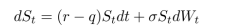
where r is the risk-free interest rate and W is a Wiener process under the risk-neutral probability measure.

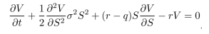
We know that the price of the option, V (S, t), on the above stock satisfies the Black-Scholes (BS) equation below:

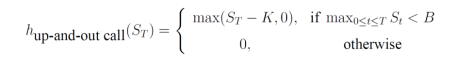
In this project you are asked to price a very popular weakly path dependent option, a Barrier option, using Finite Difference Methods (FDM). Barrier options (also called knock-in or knock-out options) are standard calls or puts except that they disappear (knock-out) or come into existence (knock-in) if the underlying asset price is found to have crossed a predetermined (barrier) level, B, at any time before the maturity of the option. They have a fairly standard naming convention which describes whether the barrier is below or above the current asset price (“down” or “up”), whether the option disappears or appears when the barrier is crossed (“out” or “in”) and whether they have a standard call or put pay-off. For instance, an up-and-out call option with zero rebate will have a payoff:

With a change of time variable τ = T – t, the equation satisfied by the option becomes:

and the payoff of a call option becomes the initial condition:

V(S, 0) = max{S – K, 0}

Let the minimum stock price be S = 0. The boundary conditions for an up-and-out call option are:
V(S = 0 , τ) = 0 ; V(S = B, τ) = 0 .

The project aims to investigate the properties of the numerical solution of the BS equation as follows:
(a) Reduce the BS equation to the heat equation (HE)
(a) Solve the HE using a Finite Difference Method (FDM) scheme of your choice; namely the explicit, the implicit, or the Crank-Nicholson scheme
(b) Use (a) and (b) to solve the BS equation numerically.

2.Project Tasks :
You are asked to implement the following programming tasks (1-5), using good coding practice (point 6 below) and to write MATLAB and PDF documentation (task 7).

1.Consider the following domain: x interval [a,b], t interval [0,T]. Generate the grid in the x, t coordinates as follows:

• Space interval divided into N equal parts (N+1 boundary points). The index values should be consistent with MATLAB array index convention running from 1 to N+1.
• Time interval divided into M equal parts (M+1 boundary points). The index values should be consistent with MATLAB array index convention running from 1 to M+1.

2.Using the change of variables described in the lectures (going from the unknown function V(S,t) to the unknown function v(x, τ) and then to the unknown function u(x, τ)), calculate the FDM grid corresponding to the conversion of the BS equation to the heat equation:

Use the values Smin = 0.001, Smax = 4 K . Write the MATLAB code to generate the x interval and the τ interval (from the values of Smin , Smax and T calculate the range of the x variable and the τ variable). Note that the change of variables is

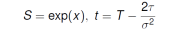
and that the above time variable is different by a factor from the time variable used in the Background section (where we used the change of time variable τ = T – t ). Calculate the corresponding grid.

3.Translate the initial and boundary conditions (1) and (2) in the correct initial and boundary conditions for the new unknown function u(x, τ).

4.Use a scheme of your choice (Implicit, Explicit, or Crank-Nicholson) to solve the heat equation for u(x, τ). In the case of the explicit finite difference scheme, demonstrate that the scheme is conditionally stable and find the condition under which the scheme would be stable.

5.Work your way back from u(x, τ) to V(S,t) to solve the Black-Sholes equation and produce:
a.a 2 d plot showing the price of the option at time 0 (on the vertical axis) vs. the stock spot price (on the horizontal axis);
b.a surface plot of the option prices V(S,t) for the whole FDM grid in S and t.

6.You can organise your code in MATLAB scrips as you prefer. Up to two marks will be awarded if: (a) you try to implement the solution as a set of MATLAB functions,wherever it helps to keep your code readable, well structured, and maintainable; (b) include MATLAB scripts calling your functions to demonstrate the code functionalities. The code
should be saved as MATLAB scripts in all cases. No code purely included as text in the documentation (with no accompanying .m file) will be considered for marking code functionalities and correctness.

7.The code should be accompanied by detailed documentation, in the form of MATLAB comments, and as typeset documents in your favourite word processing software (LaTeX, Word, etc.). Documents should be saved in PDF
format. The documentations has to consist in:

• MATLAB comments explaining the structure of the code, available functions,main variables and any other information to help to understand the code;
• developer documentation (as a typeset, not handwritten, PDF document) summarizing:
o the structure of the code, available functions, main variables and any other information to help to understand the code, including directions on how to extend the code to handle more general features;
o some numerical test runs of your code; you need to check the accuracy of your results comparing them to the values calculated using the online tool
• end-user’s instructions (as a second typeset, not handwritten, PDF document) explaining how to use the script(s), how to input data and how the results are presented, and a brief description of the methods implemented. Also, the discussions of (a) and (b) should be included here.

3.Marking :
The marks for tasks 1 to 6 will be based on coding style, clarity, and accuracy of computation. The marks for tasks 7 will be based on presentation style, clarity, and completeness of the documentation.

This project will contribute 30% towards the final mark for the module. Submit your work by uploading it in Moodle by 23:55 (UK time) on 17th of January 2022.

Submit the code as a single compressed .zip file, including all MATLAB (.m) files and the PFD files (two separate .pdf typeset documents containing developer documentation and user instructions), all residing in a single parent directory, whose name should contain your name and student code.

The project will be marked anonymously. Please do not write any information that could be used to reveal your identity in the code or in the PDF documents, or in filenames (except the .zip filename).

Unless approved mitigating circumstances apply (if you need to claim the mitigating circumstances,please refer to the mitigating circumstances procedure), late submissions will incur a penalty according to the formula:
10% × m × d, if d is less or equal to 5
100% × m, if d more than 5

Where m is the maximum mark that can be awarded for this assignment, and where d is the number of days or part days that the assignment is late, i.e., according to the standard university rules for late submission of assessed work. It is advisable to allow enough time (at least one hour) to upload your files to avoid possible congestion in Moodle before the deadline. In the unlikely event of technical problems in Moodle please email your .zip files to before the deadline.

It may prove impossible to examine projects that cannot be unzipped, opened, and run on a standard computer directly from the directories created by unzipping the submitted .zip files. In such cases a mark of 0 will be recorded. It is therefore essential that all project files and the directory structure are tested thoroughly on computer lab machines before being submitted in Moodle. It is advisable to run all such tests starting from the .zip files about to be submitted and using a different computer to that on which the files have been created.

MATLAB Compute Barrier Option Prices With Finite Difference Method Assignment – UK.

A common error is to place some files on a network drive rather than in the submitted directory. Please bear in mind that testing on a lab computer may not catch the error if the machine has access to the network drive. However, the markers would have no access to the file (since they have no access to your part of the network drive) and would be unable to compile the project. All files must be submitted inside the zipped project directory and connected to the project. Please check before submitting!

Read More :-

Question – Practical Application Of Big Data And Cloud Computing